Control Panel

After loading the data from the Excel file(s) or from the database, you can review the input data and make changes on the data pages. Before running the optimization of the model you can customize some options on the Control Panel page, such as:

Set some criteria for the constraints (Model Control)
Select objectives for the optimization model (Optimization Options)
Set data for the Custom Objective minimum required and maximum allowed (Custom Objectives Tables)
Change the considered product (Considered Product Widget)
Set the location cost and the data for open/close (Location Open/Close Data Table)
Set the minimum/maximum constraints for suppliers, production facilities, warehouses, and locations (Min/Max Constraints Table)

Model Control

In this section you can control some settings for the model to be solved by defining some criteria for the constraints. These options can be set simply by ticking some checkboxes.

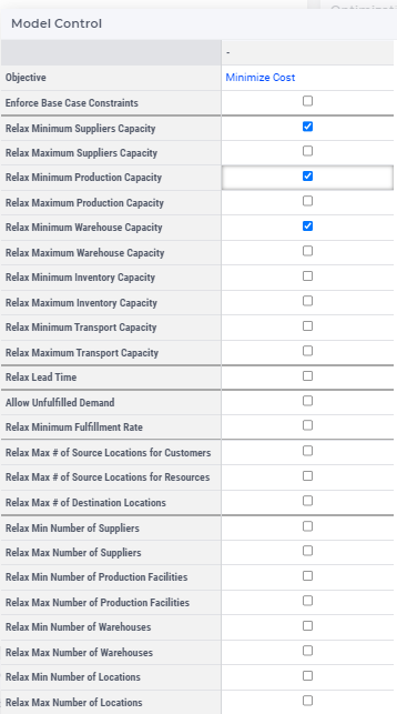
The available options which can be set are the following:

Objective: the objective of the optimization, which can be Minimize Cost, Maximize Revenue, or Maximize Profit
Enforce Base Case Constraints: when selected, the model will use Base Case Lanes and Base Case Volumes
Relax Minimum/Maximum Capacity Constraints: These options remove the constraints for minimum/maximum capacity for supply/production/warehouse/inventory/transport lane. These options allow you to see the solution if all supply/production/warehouse/inventory/transport lane had unlimited capacity. The suppliers/productions/warehouses/ transportation lanes which are above their original capacity in this solution often provide guidance on where there is most room for improvement.
Relax Lead Time: This removes the constraints for lead time, so it allows you to see how these constraint impact your solution, if at all.
Relax Minimum Lead Time Adherence: This removes the constraints for minimum lead time adherence, so it allows you to see how these constraint impact your solution, if at all. The model only takes Lead Time Adherence into account if the Lead Time is relaxed. If you select that option the Relax Lead Time option will be also selected automatically.
Allow Unfulfilled Demand: This allows for a solution in which some demand is not fulfilled.
Relax Minimum Fulfillment Rate : This removes constraints for minimum fulfillment rate.
Relax Max number of Source Locations for Customers/Resources: These options removes the constraints for the maximal number of source locations for customers/warehouses/production facilities.
Relax Max number of Destination Locations: This removes the constraints for the maximal number of destination locations.
Relax Mininmum/maximum Number of Suppliers/Production Facilities/Warehouses/Locations: These options remove the constraints for the minimal/maximum number of suppliers/production facilities/warehouses/locations.
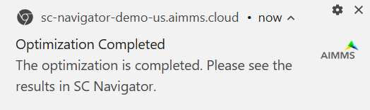
Solve in Background: This option allows that the optimization process is running in the background, allowing you to continue to use SC Navigator, including starting other solves. The progress of the optimization process will be visible on the status bar, from where you can also load the results once they are available. When this option is off, the SC Navigator app will be in ‘running’ mode during the optimization and you can only wait for its completion. After that, results are loaded automatically.
Allow Notification after Optimization : This option allows you to get a Windows notification when the optimization is finished. Note that if you start multiple runs, the notification will only appear when all runs are finished.

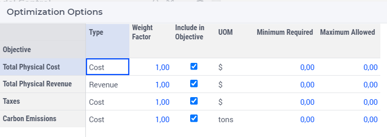
Optimization Options

The Optimization Options table contains all possible objectives which can be selected for the optimization, namely:

Total Physical Cost
Total Physical Revenue
Custom Objectives

Next we discuss each of the columns of this table in more detail.

Type Column: This column shows the type the objective. It can be cost or revenue.
Scaling Factor Column : The custom objectives may be measured in any unit and can be converted to currency by using the custom Scaling Factor.
Include in Model Objective Column:
- You can choose to select only one objective by ticking in its checkbox in the Include in Model Objective column. In this case, the value of the selected objective will be minimized/maximized.
- You can also choose to select more than one objective by ticking in their checkboxes in the Include in Model Objective column. The model will try and make a trade off between the selected objectives during the optimization.
- Even if an objective is not selected, it will be still calculated, but not minimized/maximized.
UOM Column: This column shows which unit of measurement (UOM) belongs to the objective.
Minimum Required Column: You can set restrictions on the values of the physical cost, the physical revenue, and the custom objectives. You can choose to impose a constraint for an objective by setting a lower bound in its row in the Minimum Required column of the table.
Maximum Allowed Column: You can set restrictions to the values of physical cost, physical revenue and custom objectives. You can choose to set a constraint for an objective by setting an upper bound in its row in the Maximum Allowed column of the table. You can set restrictions to the values of physical cost, physical revenue and custom objectives. You can choose to set a constraint for an objective by setting an upper bound in its row in the Maximum Allowed column of the table.
Total Value Column : After the optimization has been completed the Total Value column appears in the table and shows the solution.

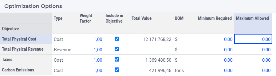
Note

The Total Value is given in the units of measurements (UOM) of the objective, which can be found in the UOM column, next to the Total Value column.

Custom Objectives Tables

There are several types of custom objectives tables which we discuss in turn below. In these tables the custom objectives ordered by different aspects, like activity type, location, mode of transport. You can set constraints for each custom objective in these tables. The use of tables will be shown in the Custom Objectives by Activity Type table.

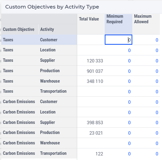
Custom Objectives by Activity Type Table

In this table the custom objectives are ordered by the activity type they belong to. Activity type can be one of the following: supplier, production, warehouse, and customer.

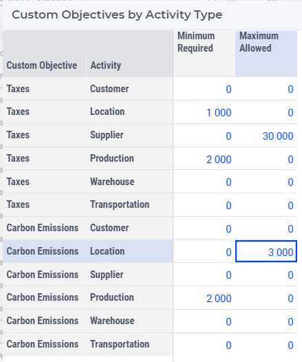
You can set constraints for each custom objective by setting a lower or an upper bound in its row in the Minimum Required or Maximum Allowed column, respectively. After the optimization has been completed, this table shows an overview of the custom objectives, including their Total Values, Minimum Required and Maximum Allowed data.

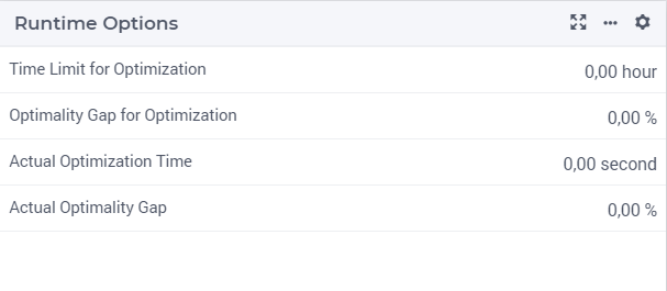
Runtime Options Table

In this table you can see the input solver options, such as the Time Limit for Optimization and the Optimality Gap for Optimization, and their values after the optimization.

Note

Time limit: The time limit of the optimization run measured in hours. If not specified, the model uses 1 hour. If specified, the data comes from the attribute “Time Limit”.
Optimality Gap: The optimization engine stops when a solution is found which is within this percentage of the best possible solution. The default is 0.01(%) when using Single Source and 0.001(%) otherwise. If specified, these data come from attribute “Optimality Gap”.

SC Navigator will return the best solution found within the time limit. The Actual Optimization Time and Actual Optimization Gap show the actual values, which can be compared to the limits above.

Location Open/Close Data Table

In the table Location Open/Close Data you can set constraints for locations, such as:

Add fixed costs
Set force open/close data
Add fixed cost/revenue for custom objective

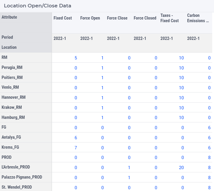
All the locations you can found in the row headers and all the attributes can be found in the column headers. You can modify the data by overwriting the numbers marked in blue.

Min/Max Constraints Table

In the table Min/Max Constraints you can set constraints involving minimum and maximum numbers of locations/suppliers/productions/warehouses. For example, if you set the maximum number of suppliers to 20, the model can use only 20 suppliers.

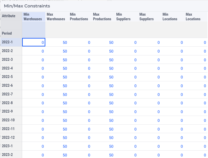
All the periods can be found in the row headers and all the attributes can be found in the column headers. You can add or change the constraints by rewriting the numbers marked in blue.