E2E Lead Time
This functionality enforces a constraint on the total end-to-end lead time (E2E Lead Time) within the supply chain network, ensuring that the cumulative time spent across all stages - including supplier, production, warehouse, and transportation - does not exceed a specified limit.
The E2E Lead Time includes:
Supplier Lead Time
Production Lead Time
Warehouse Lead Time
Transportation Lead Time.
The customer’s specified limit is:
Maximum E2E Lead Time
Above attributes are described in End-to-End (E2E) Lead Time Attributes.
Note
Using this functionality can be highly resource-intensive. Therefore, the option is disabled by default to prevent accidental use. You can enable it by using “Enforce E2E Lead Time Constraints” in Settings sheet or on the Control Panel page.
E2E Lead Time Constraints
An additional layer of constraint is applied to ensure that:
Supplier Lead Time + Production Lead Time + Warehouse Lead Time + Transportation Lead Time ≤ Maximum E2E Lead Time
Enforcing these constraints significantly increases the computational complexity of the supply chain network optimization model. The model must track and sum lead times across multiple stages (supplier - production - warehouse - transportation) for every feasible flow path and product. This introduces many additional variables and constraints that link multiple nodes and arcs in the network.
Solving with E2E Lead Time Constraints
This section describes the iterative process used by the model to optimize solutions while satisfying end-to-end (E2E) lead time constraints.
To avoid unnecessary performance overhead that would result from applying E2E lead time constraints to all demand points at once, the model adopts an iterative and selective approach. It begins with an optimization run that includes all standard constraints but excludes the E2E lead time constraint. Based on the resulting solution, E2E lead time compliance is evaluated, and constraints are incrementally introduced only where violations occur. This iterative approach continues until all violations are resolved or the solution converges.
Step-by-Step Process
Initial Optimization (Without E2E Lead Time Constraints)
The model first runs an optimization without applying any E2E lead time constraints. This provides a baseline optimized solution based purely on standard constraints such as capacity limits, cost or other objective functions.
E2E Lead Time Calculation
For each demand point, the model calculates the E2E lead time based on the results from the initial optimization.
Validation of Lead Time Compliance
If all demand points satisfy the E2E lead time constraint, the current solution is considered valid and the process ends.
If any demand points exceed the allowed E2E lead time, these are identified as violations and will trigger the next step.
Constraint Application and Re-optimization
The model applies E2E lead time constraints to the violating demand points only. It then re-runs the optimization with these additional constraints in place.
Iterative Refinement
- After re-optimization, the model recalculates the E2E lead times for all demand points. The following outcomes are possible:
No violations remain: The optimized solution is final and valid.
Same set of violations persist: The model concludes that no further improvement is achievable under the given parameters.
New violations appear: These new demand points are added to the set of constrained points, and the optimization is repeated from Step 4.
This iterative cycle continues until all E2E lead time violations are resolved or the model converges on a solution that cannot be further improved.
E2E Lead Time Page
Once optimization solution is available, a page called “E2E Lead Time” ![]() appears in the Results workflow. This page presents the detailed output from E2E Lead Time model, summarizing how demand is fulfilled across the supply chain while respecting lead time constraints.
appears in the Results workflow. This page presents the detailed output from E2E Lead Time model, summarizing how demand is fulfilled across the supply chain while respecting lead time constraints.
To illustrate, consider the demand point (Aalborg, Aalborg, Mono-Crystalline, 2023-CY). In the table below, all rows beginning with (2023-CY, Aalborg, Aalborg, Mono-Crystalline) represent the flow components contributing to this demand’s fulfillment.
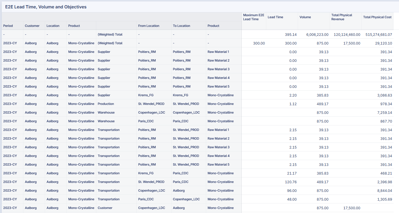
Column Descriptions
Maximum E2E Lead Time - The maximum allowable total lead time specified for the customer’s demand.
Lead Time - The time incurred at each stage of the supply chain:
For Supplier, Production, and Warehouse stages, the From Location and To Location are the same, representing the time required to process or handle the material at that facility.
For Transportation, the Lead Time represents the transit duration along each lane.
Volume - The quantity of material or product flowing through each node or transportation lane in the supply chain.
Total Physical Revenue - The revenue generated from the corresponding volume at that stage.
Total Physical Cost - The cost incurred for processing or transporting the corresponding volume.
At the top of the table, the (Weighted) Total Lead Time value (e.g., 395.14) represents the volume-weighted average lead time across all demand points in the network.
This table allows users to trace how the total lead time is accumulated across suppliers, production sites, warehouses, and transportation routes, ensuring that the final delivery to the customer remains within the defined Maximum E2E Lead Time.
Applicability and typical use cases
This feature best fits:
Make-to-Order environments where customer-specific paths must meet a promised lead time.
Long lead time supply chains (e.g., computer chips, chemicals, pharmaceuticals) where upstream stages significantly impact delivery time.
Scenarios where the trade-off between carrying inventory and meeting strict E2E lead time targets is important.
Additional Rules and Data Validation
Lead Time Aggregation in Bill of Materials (BOM)
The calculated E2E Lead Time for final products is based on the sum of lead times from all raw materials in the Bill of Materials (BOM). Below are three specific use cases for lead time aggregation in BOMs:
Use Case 1: For Bill of Material that creates number of final product less than the number of needed raw product units: 1+1 -> 1.
Use Case 2: For Bill of Material that creates number of final product equal to the number of needed raw product units: 1+1 -> 2.
Use Case 3: For Bill of Material that creates number of final product more than the number of needed raw product units: 1+1 -> 3.
In the table below, BOM_A is an example of Use Case 1, BOM_B is an example of Use Case 2, BOM_C is an example of Use Case 3.
Bill of Material |
Product |
Period |
Product Created |
Product Needed |
|---|---|---|---|---|
BOM_A |
Product A |
2023 |
1 |
|
BOM_A |
Product D |
2023 |
1 |
|
BOM_A |
Product E |
2023 |
1 |
|
BOM_B |
Product B |
2023 |
2 |
|
BOM_B |
Product D |
2023 |
1 |
|
BOM_B |
Product E |
2023 |
1 |
|
BOM_C |
Product C |
2023 |
3 |
|
BOM_C |
Product D |
2023 |
1 |
|
BOM_C |
Product E |
2023 |
1 |
As part of input data, the Supply, Production, Warehouse, and Transportation lead times are all 1.
The screenshot below shows the E2E Lead Time results:
Product A: 8.00.
Product B: 5.50
Product C: 4.67
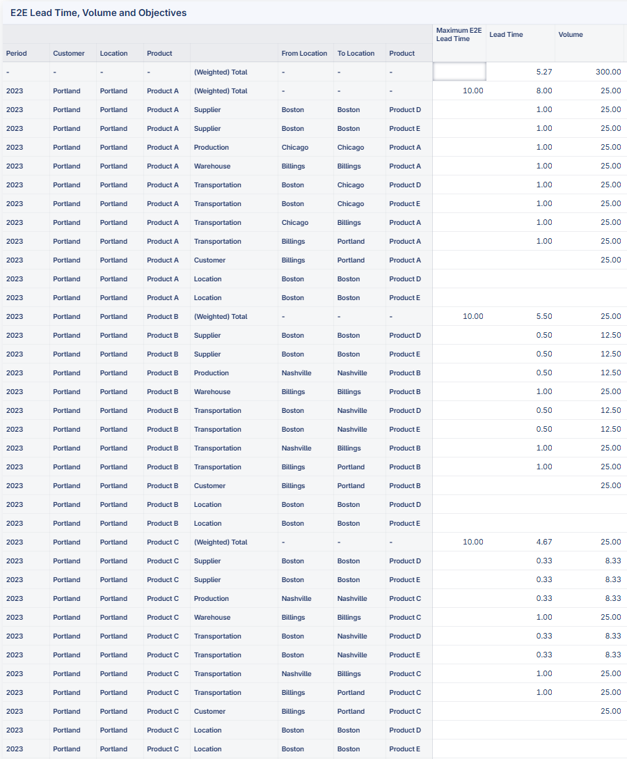
The breakdown of lead time calculation is as follows:
For all three products, the warehouse lead time and transportation lead time for final product are 3.
- Product A:
Supply lead time for raw material is 1+1=2
Production lead time is 1
Transportation lead time for raw material is 1+1=2
Total E2E Lead Time is 3+2+1+2=8.
- Product B:
Supply lead time for raw material is (1+1)/2=1
Production lead time is 1/2=0.5
Transportation lead time for raw material is (1+1)/2=1
Total E2E Lead Time is 3+1+0.5+1=5.5
- Product C:
Supply lead time for raw material is (1+1)/3=0.67
Production lead time is 1/3=0.33
Transportation lead time for raw material is (1+1)/3=0.67
Total E2E Lead Time is 3+0.67+0.33+0.67=4.67
Data validation:
A warning message is raised if number of units in product created and product needed are not equal: “WARNING: Number of units in product created and needed in Bill of Materials are not equal. The calculated E2E lead time can be underestimated/overestimated.”
Single layer BOM
Model recommendations for multi-layer BOM:
Create a dummy location for each layer of BOM.
Data validation:
An error message will be raised.
One product created in each BOM
Model recommendations for multiple products created per BOM:
Create a dummy BOM for each product created.
Data validation:
An error message will be raised.
One type of entity at one location
Model recommendations for multiple types of entity at one location:
Create a dummy location for each type of entity.
Data validation:
An error message will be raised.
No opening inventory
Data validation:
An error message will be raised.
Not compatible with multi-period modeling
Data validation:
An error message will be raised.
Other limitations
Circular flow model doesn’t suit for E2E lead time feature. It’s not prevented, but not recommended to use circular flow with E2E lead time feature.